
Timescales
Time-Duration and Time-Date: the hourglass and the calendar
Time has two meanings: it could be either duration or date. Duration represents two dates difference: it corresponds to the date differential. Similarly, by integrating constant durations, one can spot the date. Historically, time has been measured with date-indicating instruments, such as the calendar and sundial, and fixed durations accumulating instruments, such as hourglass or clepsydra (water clock).
This difference corresponds to the more recent time unit and timescale notions:
- a time standard defines the unit of duration: the second;
- a clock counts time units and characterizes a date: the timescale.
A modern timescale should check four qualities:
- Durability: a timescale should continue to date all future events.
- Accessibility – Universality: a timescale should be accessible to all potential users.
- Stability: the duration of the time unit should be constant over time.
- Accuracy: the duration of the time unit should be equal to its definition.
For example, a clock that realizes time units always strictly equal to 0.9 seconds is perfectly stable but very inaccurate. Conversely, a clock whose realization of the time unit varies from 0.9 s to 1.1 s but whose average is precisely 1 s, is very unstable but accurate. We also often distinguish short-term stability (property of a clock whose realization of the time unit varies very little over short times, but evolves slowly over time) and long-term stability (property of a clock whose realization of the time unit varies a lot over short times, but whose average changes little over time).
Old Timescales
First definition of the second (official definition of the second in the International System of Units until 1960):
The second is the 1/86400th part of the mean solar day.
The corresponding timescale is Universal Time (UT):
Universal Time UT is the mean solar time for the prime meridian increased by 12 hours.
Strictly speaking, solar time is not a time, but an angle: the true solar time at a given location and time is the hourly angle of the Sun at that place and at that time. But this angle increases (almost) in proportion to time.
In fact, UT definition does not involve the true solar time but the mean solar time. True solar time fluctuates over time mainly due to two phenomena:
1. Earth’s orbit is an ellipse. Earth’s motion around the Sun, thus the apparent movement of the Sun in the sky, varies according to the proximity of the Sun, faster in January when the Earth is at perihelion, slower in July when the Earth is at aphelion. Therefore, the true solar day length is shorter in January and longer in July (note that this effect is not related to days are longer in summer than in winter!). This variation of the true solar day has therefore a period of one year.
2. The solar day length is determined by the projection of the Sun’s motion onto the celestial equator. At the solstices, the Sun moves parallel to the celestial equator while at the equinoxes its displacement is inclined by 23° 27′ with respect to the celestial equator. Thus, the geometric projection of the Sun onto the equator moves faster at solstices than at equinoxes. Therefore, the corresponding variation of the true solar day has a period of six months.
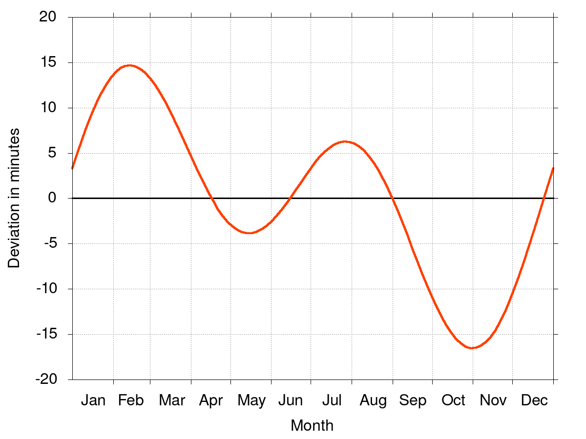
The mean solar time represents the true solar time without these fluctuations. The latter, which accumulated over one year reach an amplitude of about twenty minutes, can indeed be easily calculated and thus corrected: this is the equation of time (see Figure 1), well known to sundial enthusiasts.
Universal Time determination:
In practice, universal time is determined by writing down the instant of the meridian (North-South plane) transit of stars with known coordinates. Such a measurement actually gives sidereal time that will then have to convert into a first universal timescale, UT0, which is in a way “raw universal time”. The last step is to calculate the instantaneous Earth rotation axis (the North Pole, for example, moves on the Earth surface by several meters per year) and also the universal time referred to this instantaneous rotation axis: UT1, which is more accurate than UT0, was the official time scale until 1960. It required the assistance of a large number of observatories, both for the determination of the sidereal time and for the calculation of the Earth instantaneous rotation axis position.
Uncertainty on the Universal Time determination:
In real time, UT0 can be accessed with some 0.1 second accuracy. After correction (2 months later), UT1 is given with about 1 ms uncertainty (1 millisecond = 0.001 second). It is then necessary to correct the date of all the events identified on the raw timescale.
While this timescale could seem sufficient for most of the needs of this time, its irregularities had been reported as early as 1929. Particularly, in addition to random fluctuations in the day length, an annoying phenomenon had already been detected: the duration of the mean solar day, and therefore of the UT1’s second, tends to increase by about ten milliseconds per century, thus derogating from the principles of durability and stability that a timescale must follow. This slowdown in the Earth’s rotation is due to the Moon’s attraction and results from energy losses by tidal effects. During the time of the dinosaurs, for example, the day length was about twenty hours. It will stabilize in a few billion years, when the Earth will show always the same face to the Moon, i.e., a duration of the day equivalent to current 28 days! Notice this same effect makes the Moon to always show us the same face: the Moon being lighter, has stabilized much faster than the Earth.
Anyway, a new and more stable timescale should be used. In 1956, the International Committee of Weights and Measures (CIPM) decided to use the Earth revolution around the Sun as the basis of a new timescale, called Ephemeris Time. This definition was ratified by the 11th General Conference on Weights and Measures (CGPM) in 1960.
Second definition of the second (from 1960 to 1967):
The second is the fraction 1/31,556,925.9747 of the tropic year for January 0, 1900 at 12 hours ephemeris time.
The corresponding timescale is the Ephemeris Time (TE):
The Ephemeris Time TE is computed as a solution of the equation giving the geometric mean longitude of the Sun:
L = 279°41’48,04″ + 129.602.768,13″ T + 1,089″ T2
where T is in Julian centuries of 365,25 days of the ephemeris. T origin is dated January 0, 1900 at 12 hours TE, at the instant when the Sun mean longitude took the value 279°41’48.04″. Depending on the ideal time T of mechanics, the Sun geometric mean longitude is therefore expressed by a quadratic equation: there is identification between this T parameter of the equation and TE.
Ephemeris Time determination:
In theory, the ephemeris time is obtained by measuring the Sun position with respect to stars with known coordinates. In practice, such a measurement obviously cannot be carried out directly. In fact, TE determination was performed by measuring the Moon position with respect to stars with known coordinates, after standardizing this secondary clock respectively to the Sun movement in longitude.
Uncertainty on Ephemeris Time determination:
The main disadvantage of TE is that it takes at least a year for the inaccuracy measurements to not be excessive (on the order of 0.1 s). It is determined, in the short term, with a much lower precision than UT.
On the other hand, it has a very good long-term stability: about a few 10-9 (or 1 second in 10 years). Note that the definition of the TE second involves the too abstract 1900 tropic year, and contradicts properties of durability and accessibility-universality that a timescale has to respect. In fact, its use has been limited to astronomical needs only and has never been used in everyday life.
Moreover, in the brief years when TE was the official timescale (and even before), technological advancements in the design and construction of atomic clocks foreshadowed a limited future for this timescale. Indeed, in 1967, accuracy of atomic clocks reached 10-12 (1 second in 30,000 years!), which prompted the 13th General Conference on Weights and Measures to adopt the atomic second as the new unit of time.
Atomic Time
Atomic Cesium beam Clock
Atomic clock principle is based on a fundamental aspect of quantum physics: atom exist under different energy levels which are quantified, i.e., the atom energy can only take very precise values, characteristics of its nature (hydrogen, cesium, etc.), and it cannot be between these values. To move an atom from one energy level to a higher one (called atomic transition), it must receive a photon (an “elementary grain” of light) whose energy corresponds exactly to the energy difference between the final level and the initial one. Conversely, to return to the initial energy level, it has to emit itself a photon of the same energy.
However, the energy a photon is carrying is directly proportional to the associated electromagnetic wave frequency (to the color of the light). As an example, a violet light photon carries twice as much energy as a red light one, which carries more than an infra-red photon, which carries more than a radio wave photon. Let’s recall that radio waves, even not visible, are of same nature as light; only their frequency, much lower, can distinguish them.
Since the energy differences between atom states have well defined values, so does the electromagnetic wave frequency that can change its state, or be generated by its change of state. To design a clock, it is enough to use that electromagnetic wave frequency and to count its periods. Thus, similarly as a grandfather clock counts the balance oscillations (by advancing the dial hands at each period), or as a quartz clock counts quartz oscillator periods of vibrations, an atomic clock counts the electromagnetic wave periods having caused the change of atom state (passive standards) or having generated this state change (active standards).
Atomic cesium beam clock is currently the most stable and accurate atomic clock (accurate by definition, since the second is defined with respect to its operation). Its operation is illustrated in Figure 2 below, and is summarized as follows:
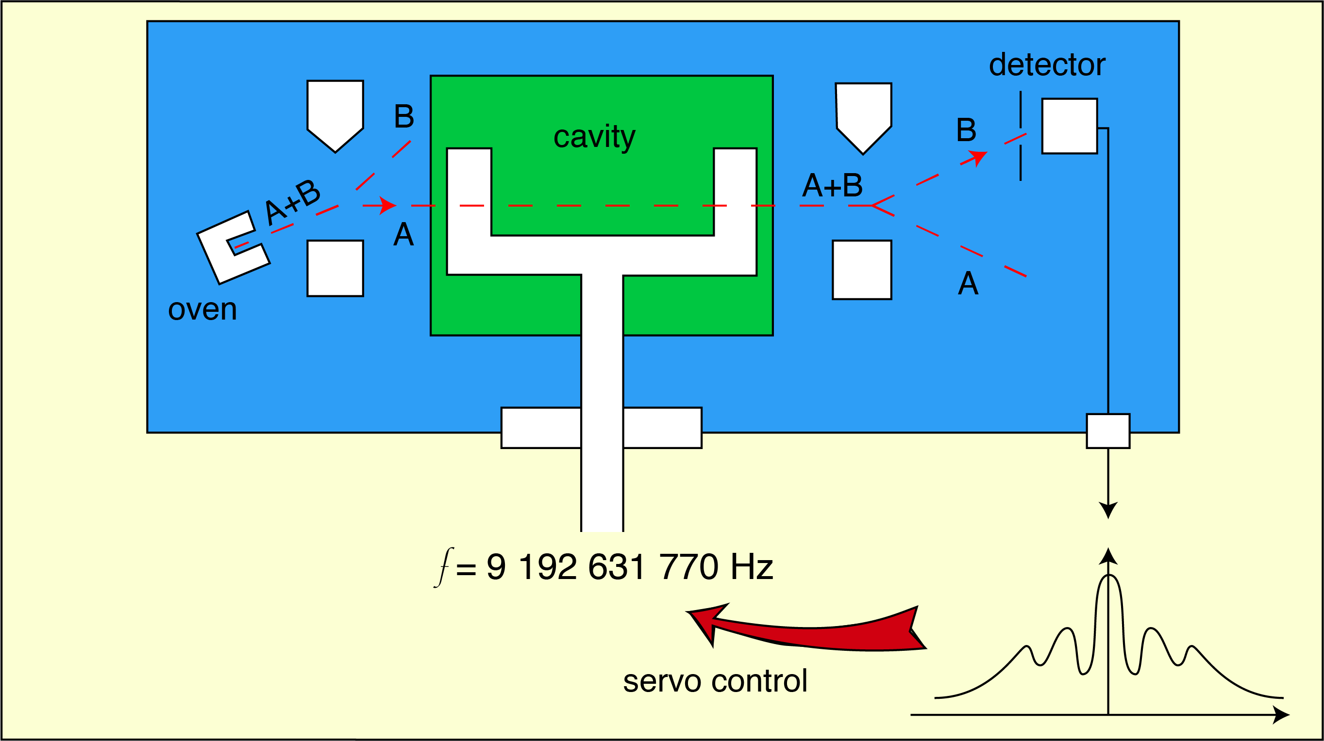
1. a crystal oscillator generates an electrical signal of frequency 10 MHz (10 megahertz, or ten million oscillations per second) as accurately as possible;
2. an electronic device multiplies the crystal oscillator signal base frequency to obtain a signal whose frequency is 9,192,631,770 Hz (frequency multiplier stage);
3. this very high frequency signal (called hyper-frequency or microwave signal) is injected into a waveguide whose geometry is such that it maintains a resonance at this particular frequency (Ramsey cavity);
4. an oven sends out a cesium-133 beam atoms, which are initially in several different energy states (symbolized by state A and state B in Figure 2);
5. a magnetic deflection system deviates atoms that are not in state A: only atoms in energy state A enter the Ramsey cavity (input selection stage);
6. if the frequency injected into the cavity is exactly 9,192,631,770 Hz, a large number of atoms go from state A to state B (interrogation phase);
7. a second magnetic deflection system separates direction of atoms in state A from that of atoms in state B (output selection stage);
8. a detector, placed in the path of atoms in state B counts the number of atoms received (detection stage);
9. depending on the detector response, a system modifies the quartz frequency so that the number of atoms detected in state B is maximum (control loop).
Note that in recent Cesium beam clocks, the magnetic deflection detection is now replaced by optical detection which has better performance for a lesser Cesium atoms flux. Thus, quartz oscillator is at the basis of an atomic cesium beam clock, the cesium atoms only helping to control and adjust the signal frequency that quartz generates: it is a passive standard.
Other types of atomic clocks exist: rubidium clocks with lesser performances, passive hydrogen masers and active hydrogen masers, with better short-term stability (durations less than one day) than cesium standards, but exhibiting poorer long-term stability (and accuracy).
The New Definition of the Second and International Atomic Time
Third definition of the second (since 1967):
The second is the duration of 9,192,631,770 radiation periods corresponding to the transition between the two hyperfine levels of Cesium 133 atom fundamental state.
International Atomic Time (TAI) is the resulting timescale:
The International Atomic Time TAI is the reference time coordinate that the International Bureau of Weights and Measures established based on the indications of atomic clocks operating in various institutions in accordance with the definition of the second, time unit, in the International System of Units.
TAI is now the official reference for dating events.
TAI Determination:
1. Each involved laboratory has to perform a local atomic timescale (accessibility): it has to possess several atomic standards (durability).
2. Local atomic timescales must be cross-comparable: each laboratory must know its local timescale advance or delay compared to those of other laboratories.
3. TAI is a weighted average of the various local atomic timescales: the weighting coefficient is determined by each local timescale performance (stability, accuracy).
4. Each laboratory receives the correspondence between its local timescale and the TAI for the elapsed period (universality): all its concerning events can be “re-dated” with respect to the TAI.
Local timescales intercomparison:
Clearly, the realization of TAI relies not only on the use of very stable and very accurate atomic standards, but also on high-performance means to intercompare the different clocks involved in the TAI design and distributed all over the Earth’s surface.
At present, intercomparisons are mainly performed through the “backwards” use of the Global Positioning System (GPS). GPS is originally a positioning system: a GPS receiver observing simultaneously 4 of GPS satellites can deduce its 3 space coordinates (latitude, longitude and altitude) and time. GPS constellation satellites are indeed equipped with atomic clocks whose signals they broadcast, and their absolute position is known at each moment. A triangulation calculation is then used to determine the receiver position.
Conversely, let’s now consider two stations, each being equipped with a GPS receiver and a local timescale. Knowing precisely the two GPS receivers position dating the same signal from a common satellite in view of these two receivers, it is possible to deduce the difference between the two stations local timescales.
Such an intercomparison is performed with an accuracy around 3 nanoseconds (3 billionths of a second).
Other much more expensive intercomparison methods, (a GPS “time” receiver costs around a few hundred €), but accurate and, above all, much greater stabilities exist. Two-way methods, for example, consisting in sending a signal from a first station to a satellite which reflects it on a second station which in turn sends it back to the first station via the satellite. Stability (reproducibility) of these methods is better than 100 picoseconds (a picosecond is worth 10-12 seconds) but its accuracy is often limited to a value of the order of one nanosecond, owing to the lack of knowledge of internal delays, in transmission and reception systems, at ground and in the satellite.
International Atomic Time instabilities estimation:
Since TAI is considered to be the most precise timescale ever at present, and, above all, TAI being the reference timescale, neither its stability nor accuracy is possible to measure (against what timescale could we perform such a measurement!). In contrast, its characteristics can be estimated if taking into account:
1. the deviation of each clock involved in the TAI with the TAI itself,
2. time transfer uncertainties.
Currently (2021), both stability and accuracy of TAI are estimated to be 10-15 (1 second per 30,000,000 years).
The atomic time revolution
Definition and use of atomic time have been a revolution in many ways:
- Timescale (time-date) is produced by “juxtaposing” the time units (time-duration) of a time-frequency standard: before then, time unit was defined as the timescale subdivision duration.
- TAI is no longer a “natural” timescale: timescales used to be directly expressed. At present, a multitude of man-made clocks are in use.
- Time becomes a physicists’ problem: it used to be an astronomers’ problem. However, several observatories continued their role of “time keepers” by acquiring atomic clocks: in particular the Besançon Observatory, faithful to its “watchmaking vocation”, the SYstèmes de Reference Temps-Espace laboratory (LNE-SYRTE) at the Paris Observatory and GÉOAZUR at the Côte d’Azur Observatory as well as, abroad, the Neuchâtel Observatory, the United States Naval Observatory (USNO), etc.
- Time (time-duration) is the most precisely determined physical quantity (≈10-15): it is the base allowing to redefine the units of other quantities. The meter definition in 1983, for example, was since based on the light travel distance in a vacuum for a period of 1 / 299,792,458 seconds: it is therefore a duration measurement that conditions accuracy of length measurements. The new definition of SI units, adopted in 2018 and in force since 2019, gives pride of place to time (and frequencies!), since the first of the 7 fundamental constants on which it is based on is the frequency of the hyperfine transition of the fundamental state of the undisturbed cesium 133 atom (9 192 631 770 Hz). All SI units now depend more or less directly on it.
The adoption of TAI resulted in a gain in stability and accuracy of more than 4 orders of magnitude compared to previous timescales. Such a spectacular improvement has inevitably been accompanied by new difficulties.
Numerous totally negligible effects until then compared to uncertainties associated with time determination, have become very clearly noticeable. This is particularly true for relativistic effects. General relativity predicts that time flows slower near a mass, such as the Earth for example. Therefore, it is important to take into account the clock altitude (so its distance from Earth) in order to use its own time in TAI calculation. Similarly, the effect due to “black body radiation” must be corrected: any body, at a given temperature, emits radiation of a given frequency, for example infra-red at 20° C, red light at 2000° C (when a body is heated up to red), etc. The radiation the clock emits, at the laboratory temperature, interacts with the microwave wave and induces a shift in the cesium atoms transition frequency. Temperature therefore has to be measured too, in order to know the correction that has to be applied to the clock local time. About ten other effects of the same type must also be taken into account to reach degree of accuracy and stability of TAI.
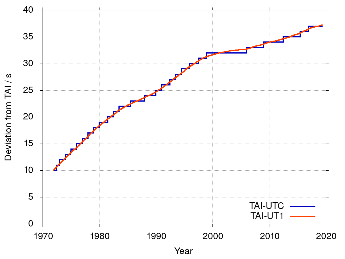
Furthermore, another drawback is directly related to the relative TAI and UT accuracies: TAI shifts with respect to UT. Yet, as UT is related to the Earth rotation and therefore to the day-night alternations, it is the timescale that naturally punctuates our lives. It is important that a timescale stays in synchronicity with it, and that noon does not strike during the night! The chosen alternative was therefore the Coordinated Universal Time (UTC) which follows TAI, and thus has both the same stability and accuracy, without ever deviating from UT1 by more than 0.9 seconds. How to succeed in such operation? By adding a “leap second” to UTC as soon as needed (see figure 3)! The last intercalated second was added between December 31, 2016 at 11:59:59 p.m. and January 1, 2017 at 12:00 a.m.; the seconds succession was: 23h59m59s, 23h59m60s, 0h0m0s.
UTC is in fact used to generate all countries legal time.
F. Vernotte, May 19 2021